Each time you work with spreadsheets, you will inevitably be working with formulas at some point. The challenge with formulas is knowing where they are being used and how to view them to streamline your data analysis. The ability to quickly visualize and analyze formulas, check for errors, and compare formulas can enhance your productivity and gain valuable insights.
Built-in Excel features, such as FORMULATEXT and ‘Show Formula’ allow data analysts to view formulas easily. Other tools like ISFORMULA, the ‘CTRL + ~’ shortcut, and Conditional Formatting further aid in highlighting and displaying formulas effectively.
In this post, I will show each option in more detail and provide examples to give each option some more context.
Using the Show Formula Option
You have just received an Excel file from a fellow colleague.
The worksheet is filled with formulas, but you have no idea which cells have formulas and no idea how they work. Fear not! Excel has an in-built lifesaver for us all – the ‘Show Formulas’ option.
This often-underestimated tool can transform your approach to working with complex spreadsheets. It’s time to give it the limelight it deserves!
How to enable ‘Show Formula’?
Hidden behind the veil of Excel’s myriad features, the ‘Show Formulas’ option is a true game-changer.
It lets you peek under the hood of your spreadsheet to see the formulas in each cell instead of their results.
This powerful feature comes in handy, especially when troubleshooting or deciphering complex Excel sheets.
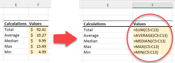
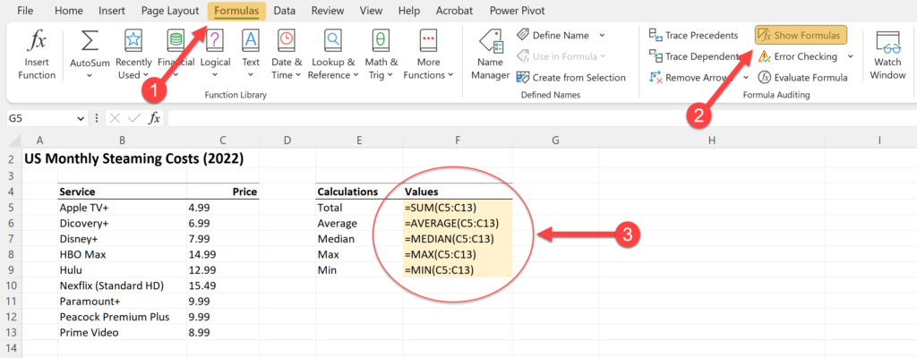
Using the ‘Show Formulas’ option is very straightforward. Follow these simple steps:
- In an open Excel spreadsheet, Navigate to the ‘Formulas’ tab.
- In the Formulas Auditing section, click on ‘Show Formulas’.
- In the spreadsheet, you will now show the underlying formula used to calculate the cell value.
But wait, there’s more! Excel has a nifty shortcut to do this even faster.
How to use the ‘CTRL + ~’ shortcut?
To activate the “Show Formulas” option without navigating through the tabs, you can use the shortcut ‘CTRL+~‘ (that’s the tilde key, just below your Escape key).
This one-step method will instantly reveal all the formulas in your spreadsheet.
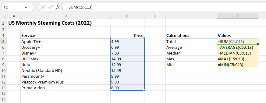
Tip:
- Use the same shortcut again to switch back to the normal view.
- The data array used in the calculation is also highlighted when selecting a cell.
Leveraging the ‘Show Formulas’ option and its shortcut can save time, increase accuracy, and improve your overall productivity.
As a user of Excel, mastering these tools empowers you to get the most out of Excel.
So let the ‘Show Formulas’ option be your secret weapon in conquering your next spreadsheet challenge! Next, we will look at leveraging conditional formatting.
How to use Conditional Formatting?
Using Excel’s Conditional Formatting is another powerful way to highlight important information and quickly visualize patterns within your datasets.
In this section, I will demonstrate how to use Conditional Formatting to show cells that contain formulas. The link below is a video demonstrating how to do this in real time.
Conditional formatting lets you dynamically format cells based on specific conditions or rules.
By applying formatting rules, you can draw attention to significant data points, identify trends, and uncover valuable insights.
In this case, we want to apply conditional formatting to a cell with a formula.
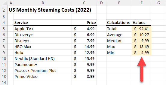
Using the ‘GO TO SPECIAL’ in Excel, you can highlight all cells containing formulas or with conditional formatting applied.
This feature provides additional customization and flexibility to your data analysis.
Here are the steps (with shortcut steps) to apply color formatting to cells with formulas in an Excel worksheet:
- Select the entire worksheet: CTRL + A + A
- Press ‘F5′ to open up the ‘Go To’ window
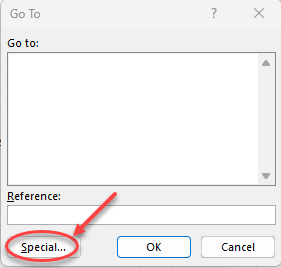
- Using the cursor and press ‘Select Special’ to open the ‘Go To Special’ window.
- Alternatively, you can use the shortcut ‘Alt + F’
- Within ‘Go To Special’ select Formula and the four sub-options. The shortcut command is ‘Alt + F’
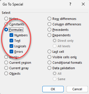
- You can keep all the check marks checked or deselect them as needed. Press ‘Enter’.
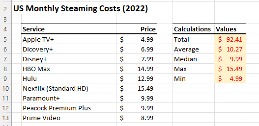
- Now within the worksheet, only the cells with formulas will be highlighted.
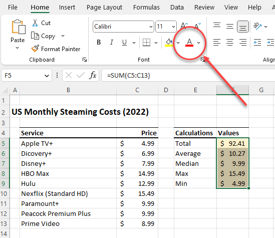
- In the Home ribbon, select the desired font color.
- It will then be applied to all the highlighted cells. (in this example, I selected red).
How to use Built-In Functions?
Lastly, Excel is renowned for its vast array of built-in functions that simplify complex calculations and streamline data analysis.
As a data analyst or in my role as a product manager, leveraging these functions can significantly boost productivity and efficiency when trying to analyze and share data.
This section’ll explore two powerful built-in functions: FORMULATEXT and ISFORMULA.
Using FORMULATEXT Function
The FORMULATEXT function is a hidden gem within Excel’s arsenal. It aims to extract the formula residing in a specified cell as text.
Watch Video – Using FormulaText Function
This function proves invaluable when working with intricate formulas or documenting your calculations.
To use it, simply follow this syntax:
=FORMULATEXT(cell_reference)
- By providing the cell_reference, the function retrieves and displays the formula text.
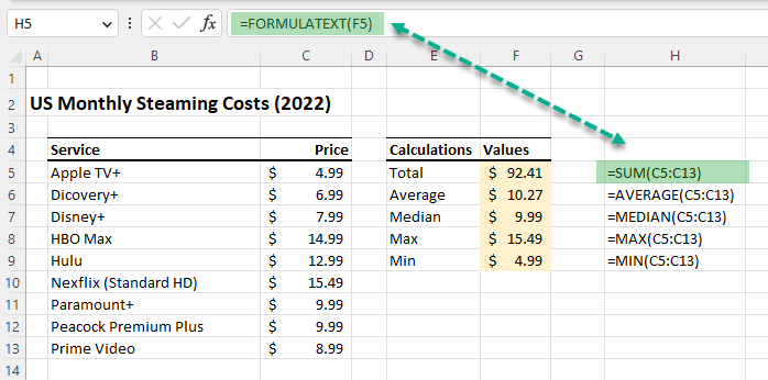
- For instance, let’s say you have a formula in cell F5 that calculates the total monthly subscription value of a group of streaming service providers.
=SUM(C5:C13)
- To extract this formula as text, you can utilize the FORMULATEXT function:
=FORMULATEXT(F5)
- The formula reveals ‘=SUM(C5:C13)’ within the designated cell, aiding understanding and documentation.
In the image below, you can see this in action:
Using ISFORMULA Function
Another handy built-in function is ISFORMULA, which allows you to determine if a cell contains a formula.
It returns TRUE if the cell contains a formula and FALSE if it doesn’t.
Here’s the syntax to employ:
=ISFORMULA(cell_reference)
Let’s consider an example.
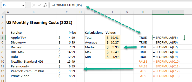
Suppose you have a dataset with formulas in column F calculating descriptive statistics for a data array.
To identify whether a cell contains a formula, implement the ISFORMULA function:
=ISFORMULA(F5)
This function yields TRUE if a formula is present in cell F5 and FALSE if it lacks a formula.
It proves particularly useful when auditing or analyzing extensive datasets.
By utilizing the power of built-in functions like FORMULATEXT and ISFORMULA, you can unravel hidden formulas, gain deeper insights, and streamline your product management tasks in Excel.
These functions empower you to optimize calculations, document formulas accurately, and analyze data.
Summary Notes:
For viewing formulas in your worksheet, the options mentioned are great to have in your data analysis tool kit. Rember:
- You can quickly view and toggle between values and formulas in a worksheet using the ‘Show Formula’ option (shortcut ‘CTRL + ~’).
- Combine that with Conditional Formatting, and you can add visual color to your analysis.
- For sharing and showing your work, using the FORMULATEXT formula is an excellent option that does not obstruct the cells with formula values.


